First Links in the Markov Chain
BY BRIAN HAYES
Probability and poetry were unlikely partners in the creation of a computational tool
COMPUTER MATHEMATICS STATISTICS
One hundred years ago the Russian mathematician A. A. Markov founded a new branch of probability theory by applying mathematics to poetry. Delving into the text of Alexander Pushkin’s novel in verse Eugene Onegin , Markov spent hours sifting through patterns of vowels and consonants. On January 23, 1913, he summarized his findings in an address to the Imperial Academy of Sciences in St. Petersburg. His analysis did not alter the understanding or appreciation of Pushkin’s poem, but the technique he developed—now known as a Markov chain—extended the theory of probability in a new direction. Markov’s methodology went beyond coin-flipping and dice-rolling situations (where each event is independent of all others) to chains of linked events (where what happens next depends on the current state of the system).
Markov chains are everywhere in the sciences today. Methods not too different from those Markov used in his study of Pushkin help identify genes in DNA and power algorithms for voice recognition and web search. In physics the Markov chain simulates the collective behavior of systems made up of many interacting particles, such as the electrons in a solid. In statistics, the chains provide methods of drawing a representative sample from a large set of possibilities. And Markov chains themselves have become a lively area of inquiry in recent decades, with efforts to understand why some of them work so efficiently—and some don’t.
As Markov chains have become commonplace tools, the story of their origin has largely faded from memory. The story is worth retelling. It features an unusual conjunction of mathematics and literature, as well as a bit of politics and even theology. For added drama there’s a bitter feud between two forceful personalities. And the story unfolds amid the tumultuous events that transformed Russian society in the early years of the 20th century.
Before delving into the early history of Markov chains, however, it’s helpful to have a clearer idea of what the chains are and how they work.Probability theory has its roots in games of chance, where every roll of the dice or spin of the roulette wheel is a separate experiment, independent of all others. It’s an article of faith that one flip of a coin has no effect on the next. If the coin is fair, the probability of heads is always 1/2.
This principle of independence makes it easy to calculate compound probabilities. If you toss a fair coin twice, the chance of seeing heads both times is simply 1/2×1/2, or 1/4. More generally, if two independent events have probabilities p and q , the joint probability of both events is the productpq .
However, not all aspects of life adhere to this convenient principle. Suppose the probability of a rainy day is 1/3; it does not follow that the probability of rain two days in a row is 1/3×1/3=1/9. Storms often last several days, so rain today may signal an elevated chance of rain tomorrow.
For another example where independence fails, consider the game of Monopoly. Rolling the dice determines how many steps your token advances around the board, but where you land at the end of a move obviously depends on where you begin. From different starting points, the same number of steps could take you to the Boardwalk or put you in jail. The probabilities of future events depend on the current state of the system. The events are linked, one to the next; they form a Markov chain.
To be considered a proper Markov chain, a system must have a set of distinct states, with identifiable transitions between them. A simplified model of weather forecasting might have just three states: sunny, cloudy and rainy . There are nine possible transitions (including “identity” transitions that leave the state unchanged). For Monopoly, the minimal model would require at least 40 states, corresponding to the 40 squares around the perimeter of the board. For each state there are transitions to all other states that can be reached in a roll of the dice—generally those from 2 to 12 squares away. A realistic Monopoly model incorporating all of the game’s quirky rules would be much larger.
Recent years have seen the construction of truly enormous Markov chains. For example, the PageRank algorithm devised by Larry Page and Sergey Brin, the founders of Google, is based on a Markov chain whose states are the pages of the World Wide Web—perhaps 40 billion of them. The transitions are links between pages. The aim of the algorithm is to calculate for each web page the probability that a reader following links at random will arrive at that page.
Past, Present and Future
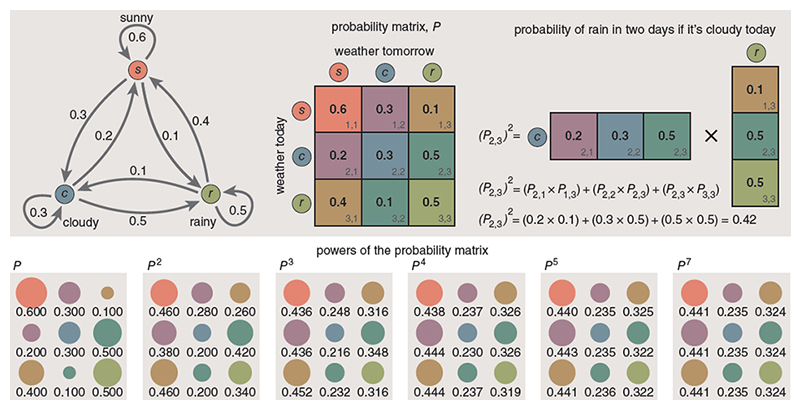
A diagram made up of dots and arrows shows the structure of a Markov chain. Dots represent states; arrows indicate transitions. Each arrow has an associated number, which gives the probability of that transition. Because these numbers are probabilities, they must lie between 0 and 1, and all the probabilities issuing from a dot must add up to exactly 1. In such a diagram you can trace a pathway that defines a sequence of states—perhaps sunny, sunny, cloudy, rainy in the weather example. To calculate the probability of this specific sequence, just multiply the probabilities associated with the corresponding transition arrows.The chain can also answer questions such as, “If it’s cloudy today, what is the probability of rain two days from now?” The answer is found by summing the contributions of all pathways that lead from the cloudy state to the rainy state in exactly two steps. This sounds like a tedious exercise, but there’s an easy way to organize the computation, based on the arithmetic of matrices.

Illustration by Brian Hayes.
The transition probabilities for a three-state Markov chain can be arranged in a three-by-three matrix—a square array of nine numbers. As shown in the illustration at right, the process for calculating multistage transitions is equivalent to matrix multiplication. The matrix itself (call it P ) predicts tomorrow’s weather; the product P × P , or P 2 , gives weather probabilities for the day after tomorrow; P 3 defines the probabilities for three days hence, and so on. The entire future unfolds from this one matrix.
Given the hypothetical probabilities in the weather example shown at right, the successive powers of the matrix rapidly converge to a stationary configuration in which all the rows are identical and all the columns consist of a single repeated value. This outcome has a straightforward interpretation: If you let the system evolve long enough, the probability of a given state no longer depends on the initial state. In the case of the weather, such a result is unsurprising. Knowing that it’s raining today may offer a clue about tomorrow’s weather, but it’s not much help in predicting the state of the skies three weeks from now. For such an extended forecast you may as well consult the long-term averages (which are the values to which the Markov chain converges).
Markov’s scheme for extending the laws of probability beyond the realm of independent variables has one crucial restriction: The probabilities must depend only on the present state of the system, not on its earlier history. The Markovian analysis of Monopoly, for example, considers a player’s current position on the board but not how he or she got there. This limitation is serious. After all, life presents itself as a long sequence of contingent events—kingdoms are lost for want of a nail, hurricanes are spawned by butterflies in Amazonia—but these causal chains extending into the distant past are not Markov chains.
On the other hand, a finite span of history can often be captured by encoding it in the current state. For example, tomorrow’s weather could be made dependent on both yesterday’s and today’s by creating a nine-state model in which each state is a two-day sequence. The price to be paid is an exponential increase in the number of states.
Peterburgian Math
In trying to understand how Markov came to formulate these ideas, we run straight into one of those long chains of contingent events extending deep into the past. One place to start the story is with Peter the Great (1682–1725), the ambitious Romanov tsar who founded the Academy of Sciences in St. Petersburg and fostered the development of scientific culture in Russia. (Other aspects of his reign were less admirable, such as the torture and murder of dissidents, including his son Alexei.)
At roughly the same time, elsewhere in Europe, the theory of probability was emerging from gambling halls and insurance brokerages to become a coherent branch of mathematics. The foundational event was the publication in 1713 of Jacob Bernoulli’s treatise Ars Conjectandi ( The Art of Conjecturing ).
Back in St. Petersburg, the mathematics program prospered, although initially most of the accomplishments were by imported savants. Visitors to the Academy included two younger members of the Bernoulli family, Nicholas and Daniel. And the superstar was Leonhard Euler, the preeminent mathematician of the era, who spent more than 30 years in St. Petersburg.
By the 19th century indigenous Russian mathematicians were beginning to make their mark. Nikolai Lobachevsky (1792–1856) was one of the inventors of non-Euclidean geometry. A few decades later, Pafnuty Chebyshev (1821–1894) made contributions in number theory, in methods of approximation (now called Chebyshev polynomials) and in probability theory. Chebyshev’s students formed the nucleus of the next generation of Russian mathematicians; Markov was prominent among them.

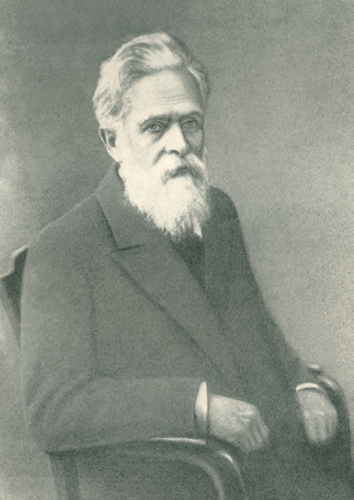
From A. A. Markov, 1926.
Andrei Andreevich Markov was born in 1856. His father was a government employee in the forestry service and later the manager of an aristocrat’s estate. As a schoolboy Markov showed enthusiasm for mathematics. He went on to study at St. Petersburg University (with Chebyshev and others) and remained there for his entire career, progressing through the ranks and becoming a full professor in 1893. He was also elected to the Academy.
In 1906, when Markov began developing his ideas about chains of linked probabilities, he was 50 years old and had already retired, although he still taught occasional courses. His retirement was active in another way as well. In 1883 Markov had married Maria Valvatieva, the daughter of the owner of the estate his father had once managed. In 1903 they had their first and only child, a son who was also named Andrei Andreevich. The son became a distinguished mathematician of the Soviet era, head of the department of mathematical logic at Moscow State University. (To the consternation of librarians, both father and son signed their works “A. A. Markov.”)
An intellectual thread extends all the way from Jacob Bernoulli through Chebyshev to Markov. In Ars Conjectandi Bernoulli stated the law of large numbers, which says that if you keep flipping an unbiased coin, the proportion of heads will approach 1/2 as the number of flips goes to infinity. This notion seems intuitively obvious, but it gets slippery when you try to state it precisely and supply a rigorous proof. Bernoulli proved one version; Chebyshev published a broader proof; Markov offered further refinements.
Markov’s later studies of chains of dependent events can be seen as a natural continuation and generalization of this long line of work. But that’s not the whole story.
Mathematical Theology
By most accounts, Markov was a nettlesome character, abrasive even with friends, fiercely combative with rivals, often embroiled in public protests and quarrels. We get a glimpse of his personality from his correspondence with the statistician Alexander Chuprov, which has been published in English translation. His letters to Chuprov are studded with dismissive remarks denigrating others’ work—including Chuprov’s.
Markov’s pugnacity extended beyond mathematics to politics and public life. When the Russian church excommunicated Leo Tolstoy, Markov asked that he be expelled also. (The request was granted.) In 1902, the leftist writer Maxim Gorky was elected to the Academy, but the election was vetoed by Tsar Nicholas II. In protest, Markov announced that he would refuse all future honors from the tsar. (Unlike Anton Chekhov, however, Markov did not resign his own membership in the Academy.) In 1913, when the tsar called for celebrations of 300 years of Romanov rule, Markov responded by organizing a symposium commemorating a different anniversary: the publication ofArs Conjectandi 200 years before.
Markov’s strongest vitriol was reserved for another mathematician, Pavel Nekrasov, whose work Markov described as “an abuse of mathematics.” Nekrasov was on the faculty of Moscow University, which was then a stronghold of the Russian Orthodox Church. Nekrasov had begun his schooling at a theological seminary before turning to mathematics, and apparently he believed the two vocations could support each other.
In a paper published in 1902 Nekrasov injected the law of large numbers into the centuries-old theological debate about free will versus predestination. His argument went something like this: Voluntary acts—expressions of free will—are like the independent events of probability theory, with no causal links between them. The law of large numbers applies only to such independent events. Data gathered by social scientists, such as crime statistics, conform to the law of large numbers. Therefore the underlying acts of individuals must be independent and voluntary.
Markov and Nekrasov stood at opposite poles along many dimensions: A secular republican from Petersburg was confronting an ecclesiastical monarchist from Moscow. But when Markov launched his attack on Nekrasov, he did not dwell on factional or ideological differences. He zeroed in on a mathematical error. Nekrasov assumed that the law of large numbers requires the principle of independence. Although this notion had been a commonplace of probability theory since the time of Jacob Bernoulli, Markov set out to show that the assumption is unnecessary. The law of large numbers applies perfectly well to systems of dependent variables if they meet certain criteria.
Counting Vowels and Consonants

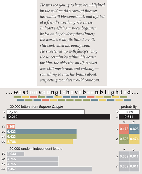
Illustration by Brian Hayes.
Markov first addressed the issue of dependent variables and the law of large numbers in 1906. He began with a simple case—a system with just two states. On the assumption that all four transition probabilities are greater than 0 and less than 1, he was able to prove that as the system evolves over time, the frequency of each state converges to a fixed average value. Over the next few years Markov extended and generalized the proof, showing that it applies to a broad class of models.
This series of results achieved at least one of Markov’s goals: It forced Nekrasov to retreat from his claim that the law of large numbers implies free will. But the wider world of mathematics did not take much notice. One thing lacking was any hint of how these ideas might be applied to practical events. Markov was proudly aloof from such matters. He wrote to Chuprov: “I am concerned only with questions of pure analysis.… I refer to the question of the applicability of probability theory with indifference.”
By 1913, however, Markov had apparently had a change of heart. His paper on Onegin was certainly a work of applied probability theory. It made a lasting impression, perhaps in part because of the novelty of applying mathematics to poetry. Perhaps too because the poem he chose is a treasured one, which Russian schoolchildren recite.
From a linguistic point of view, Markov’s analysis was at a very superficial level. It did not address the meter or rhyme or meaning of Pushkin’s verse. It treated the text as a mere stream of letters. Simplifying further still, the letters were lumped into just two classes, vowels and consonants.
Markov’s sample comprised the first 20,000 letters of the poem, which is about an eighth of the total. He eliminated all punctuation and white space, jamming the characters into one long, unbroken sequence. In the first phase of his analysis he arranged the text in 200 blocks of 10×10 characters, then counted the vowels in each row and column. From this tabulation he was able to calculate both the mean number of vowels per 100-character block and the variance, a measure of how widely samples depart from the mean. Along the way he tallied up the total number of vowels (8,638) and consonants (11,362).
In a second phase Markov returned to the unbroken sequence of 20,000 letters, combing through it to classify pairs of successive letters according to their pattern of vowels and consonants. He counted 1,104 vowel-vowel pairs and was able to deduce that there were 3,827 double consonants; the remaining 15,069 pairs must consist of a vowel and a consonant in one order or the other.
With these numbers in hand, Markov could estimate to what extent Pushkin’s text violates the principle of independence. The probability that a randomly chosen letter is a vowel is 8,638/20,000, or about 0.43. If adjacent letters were independent, then the probability of two vowels in succession would be (0.43) 2 , or about 0.19. A sample of 19,999 pairs would be expected to have 3,731 double vowels, more than three times the actual number. Thus we have strong evidence that the letter probabilities are not independent; there is an exaggerated tendency for vowels and consonants to alternate. (Given the phonetic structure of human language, this finding is not a surprise.)
Markov did all of his counting and calculating with pencil and paper. Out of curiosity, I tried repeating some of his work with an English translation of Onegin . Constructing 10×10 tables on squared paper was tedious but not difficult. Circling double vowels on a printout of the text seemed to go quickly—10 stanzas in half an hour—but it turned out I had missed 62 of 248 vowel-vowel pairs. Markov was probably faster and more accurate than I am; even so, he must have spent several days on these labors. He later undertook a similar analysis of 100,000 characters of a memoir by another Russian writer, Sergei Aksakov.
A computer reduces the textual analysis to triviality, finding all double vowels in four milliseconds. The result of such an analysis, shown in the illustration above, suggests that written English is rather vowel-poor (or consonant-rich) compared with Russian, and yet the structure of the transition matrix is the same. The probability of encountering a vowel depends strongly on whether the preceding letter is a vowel or a consonant, with a bias toward alternation.
The Bootless Academician
Markov’s Onegin paper has been widely discussed and cited but not widely read outside of the Russian-speaking world. Morris Halle, a linguist at MIT, made an English translation in 1955 at the request of colleagues who were then interested in statistical approaches to language. But Halle’s translation was never published; it survives only in mimeograph form in a few libraries. The first widely available English translation, created by the German scholar David Link and several colleagues, was published only in 2006.
Link has also written a commentary on Markov’s “mathematization of writing” and an account of how the Onegin paper came to be known outside of Russia. (A crucial figure in the chain of transmission was George Polya, a Hungarian mathematician whose well-known work on random walks is closely related to Markov chains.) The statisticians Oscar Sheynin and Eugene Seneta have also written about Markov and his milieu. Because I read no Russian, I have relied heavily on these sources.
In the accounts of Link, Seneta and Sheynin we find the dénouement of the Markov-Nekrasov conflict. Not surprisingly, the royalist Nekrasov had a hard time hanging onto his position after the 1917 Bolshevik revolution. He died in 1924, and his work fell into obscurity.
Markov, as an anti-tsarist, was looked upon more favorably by the new regime, but an anecdote about his later years suggests he remained a malcontent to the end. In 1921 he complained to the Academy that he could not attend meetings because he lacked suitable footwear. The matter was referred to a committee. In a sign of how thoroughly Russian life had been turned upside down, the chairman was none other than Academician Maxim Gorky. A pair of boots was found for Comrade Markov, but he said they didn’t fit and were “stupidly stitched.” He continued to keep his distance from the Academy and died in 1922.
The Drivel Generator

For Markov, extending the law of large numbers to interdependent samples was the main point of his inquiry. He bequeathed us a proof that a Markov chain must eventually settle down to some definite, stable configuration corresponding to the long-term average behavior of the system.
In the 100 years since 1913, Markov chains have become a major mathematical industry, but the emphasis has shifted away from the questions that most interested Markov himself. In a practical computational setting, it’s not enough to know that a system will eventually converge to a stable value; one needs to know how long it will take. With the recent vogue for huge Markov systems, even estimating the convergence time is impractical; the best that can be expected is an estimate of the error introduced by prematurely terminating a simulation process.
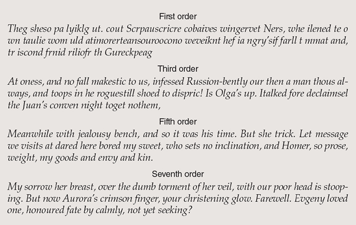
I conclude this essay with a more personal story about my own introduction to Markov chains. In 1983 I wrote a “Computer Recreations” column for Scientific American subtitled “A progress report on the fine art of turning literature into drivel.” I was exploring algorithms that exploit the statistical structure of language to generate random text in the manner of a particular author. (Some specimens based on Eugene Onegin appear in the illustration above.)
One version of the drivel algorithm builds a transition matrix whose rows are labeled by sequences of k letters and whose columns define the probabilities of various letters that can follow each k -character sequence. Given an initial k -letter seed sequence, the program uses the matrix and a random number generator to choose the next character of the synthesized text. Then the leftmost letter of the seed is dropped, the newly chosen character is appended to the right side, and the whole procedure repeats. For values of k larger than 2 or 3 the matrix becomes impractically large, but there are tricks for solving this problem (one of which eliminates the matrix altogether).
Shortly after my article appeared, I met Sergei Kapitsa, the son of Nobel laureate Pyotr Kapitsa and the editor of the Russian-language edition of Scientific American . Kapitsa told me that my algorithms for generating random text all derived from the work of A. A. Markov, decades earlier. I expressed a certain skepticism: Maybe Markov invented the underlying mathematics, but did he apply those ideas to linguistic processes? Then Kapitsa told me about Markov’s Onegin paper.
In a later issue of the magazine I published a contrite addendum about Markov. I had to write it without ever having read a word of Markov’s work, and I went overboard a little, saying that Markov “asks to what extent Pushkin’s poem remains Pushkin’s when the letters are scrambled.” Thirty years later, I hope this column will restore the balance. Sadly, though, I am too late to share it with Kapitsa. He died last summer at age 84.
'Good articles(비공개)' 카테고리의 다른 글
| Duality (0) | 2023.08.03 |
|---|---|
| The Ghost in the Quantum Turing Machine (0) | 2023.08.03 |
| What is complexity? (0) | 2023.08.03 |
| Space, time, entanglement (0) | 2023.08.03 |
| Phil Anderson’s Magnetic Ideas in Science (0) | 2023.08.03 |